Table of Contents
Markov Processes
Basically, Markov decision processes formally describe an environment for reinforcement learning, where the environment is fully observable, which means the current state completely characterises the process.
Almost all RL problems can be formalised as MDPs, e.g.
- Optimal control primarily deals with continuous MDPs
- Partially observable problems can be converted into MDPs
- Bandits are MDPs with one state
So, if we solve MDP, we can solve all above RL problems.
Markov Property
Markov Property is "The future is independent of the past given the present", like last note said. The formal definition is: \[ P[S_{t+1}|S_t]=P[S_{t+1}|S_1, ..., S_t] \] where \(S\) represents a state.
The formula means the current can capture all relevant information from the history. Once the state is known, the history may be thrown away, i.e. the state is a sufficient statistic of the future.
State Transition Matrix
We know that given the current state, we can use its information to reach the next state, but how? — It is characterized by the state transition probability.
For a Markov state \(s\) and successor state \(s'\) , the state transition probability is defined by \[ P_{ss'}=P[S_{t+1}=s'|S_t=s] \] We can put all of the probabities into a matrix called transition matrix, denoted by \(P\) : \[ P = \begin{bmatrix} P_{11} & \cdots & P_{1n} \\ \vdots & \ddots & \vdots \\ P_{n1} & \cdots & P_{nn} \end{bmatrix} \] where each row of the matrix sums to 1.
Markov Process
Formally, a Markov process is a memoryless random process, i.e. a sequence of random states \(S_1, S_2, …\) with the Markov property.
Definition
A Markov Process (or Markov Chain) is tuple \(<S, P>\)
- \(S\) is a (finite) set of states
- \(P\) is a state transition probability matrix, \(P_{ss'} = P[S_{t+1}=s'|S_t=s]\)
Example
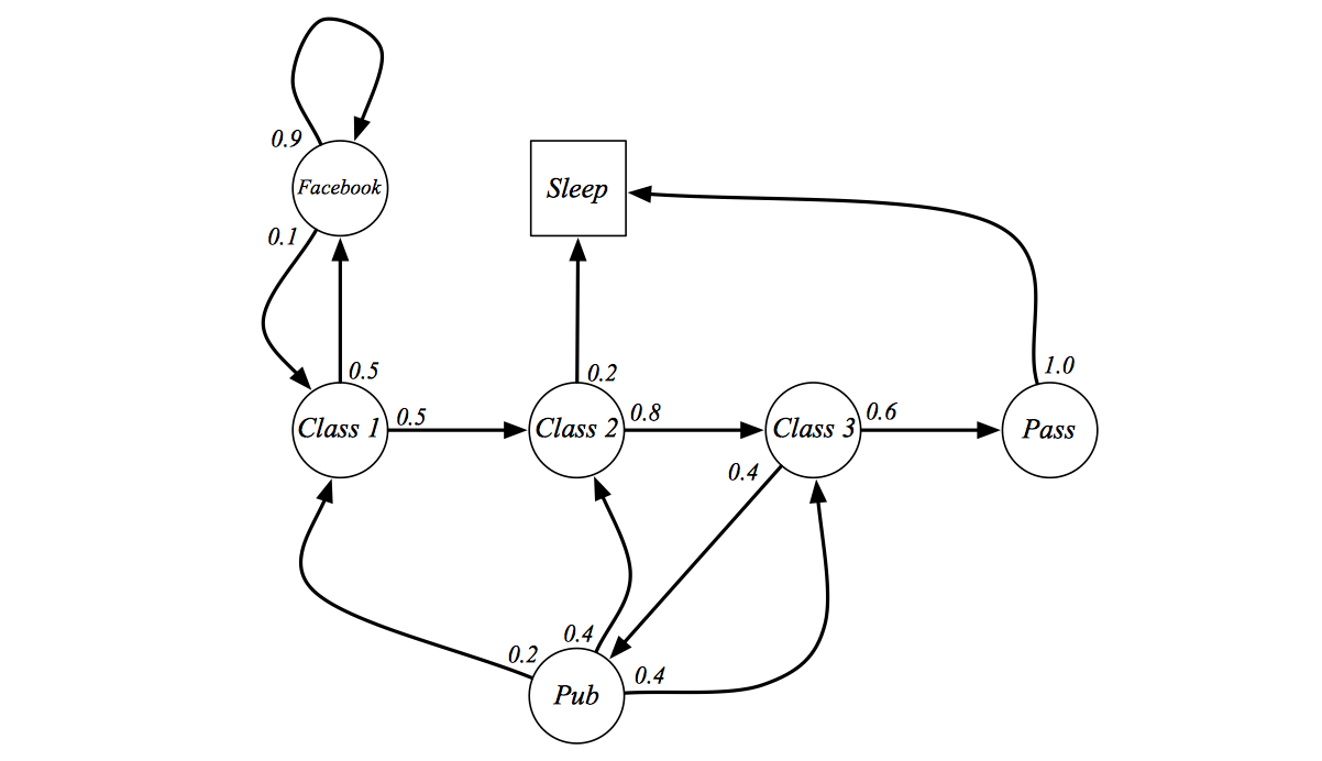
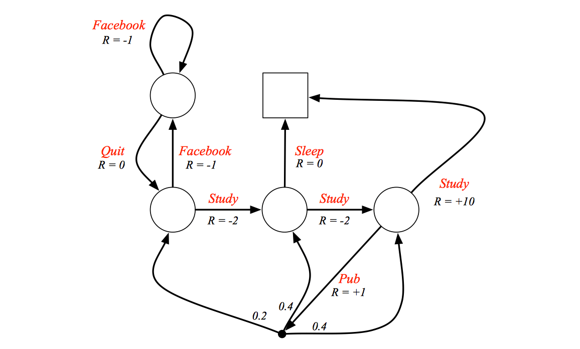
The above figure show a markov chains of a student's life. Process starts from Class 1, taking class 1 may be boring, so he have either 50% probability to look Facebook or to move to Class 2. …. And finally, he reach the final state Sleep. It's a final state just because it is a self-loop with probability 1 which is nothing special.
We can sample sequences from such process. Sample episodes for Student Markov Chain starting from \(S_1 = C_1\): \[ S_1, S_2, ..., S_T \]
- C1 C2 C3 Pass Sleep
- C1 FB FB C1 C2 Sleep
- C1 C2 C3 Pub C2 C3 Pass Sleep
- C1 FB FB C1 C2 C3 Pub C1 FB FB FB C1 C2 C3 Pub C2 Sleep
Also, we can make the transition matrix from such markov chain:
![]()
If we have this matrix, we can fully describe the Markov process.
Markov Reward Process
So far, we have never talked about Reinforcement Learning, there is no reward at all. So, let's talk about the Markov Reward Process.
The most important is adding reward to Markov process, so a Markov reward process is a Markov chain with values.
Definition
A Markov Reward Process is tuple \(<S, P, R, \gamma>\)
- \(S\) is a (finite) set of states
- \(P\) is a state transition probability matrix, \(P_{ss'} = P[S_{t+1}=s'|S_t=s]\)
- \(R\) is a reward function, \(R_s=E[R_{t+1}|S_t=s]\)
- \(\gamma\) is a discount factor, \(\gamma \in [0, 1]\)
Note that \(R\) is the immediate reward, it characterize the reward you will get if you currently stay on state \(s\).
Example
Let's back to the student example:
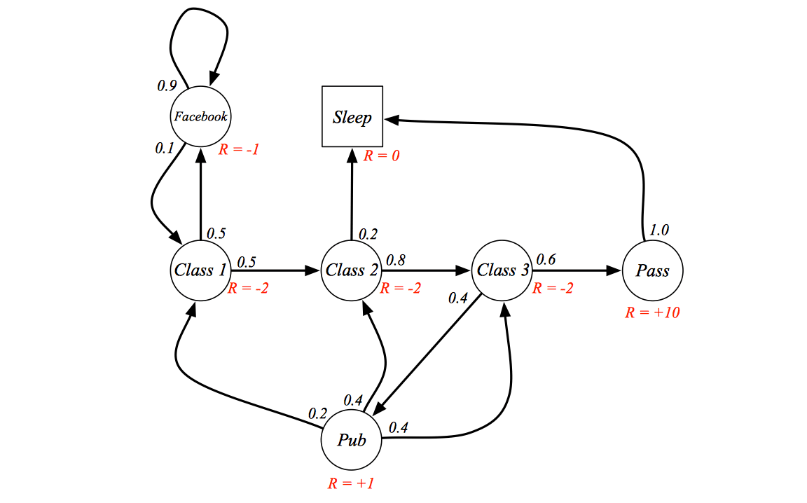
At each state, we have corresponding reward represents the goodness/badness of that state.
Return
We don't actually care about the immediate reward, we care about the whole random sequence's total reward. So we define the term return:
Definition
The return \(G_t\) is the total dicounted reward from time-step \(t\). \[ G_t=R_{t+1}+\gamma R_{t+2}+...=\sum_{k=0}^\infty \gamma^kR_{t+k+1} \]
The discount \(\gamma \in [0,1]\) is the present value of future rewards. So the value of receiving reward \(R\) after \(k+1\) time-steps is \(\gamma^k R\).
Note: \(R_{t+1}\) is the immediate reward of state \(S_t\).
This values immediate reward above delayed reward:
- \(\gamma\) closes to \(0\) leads to "myopic" evaluation
- \(\gamma\) closes to \(1\) leads to "far-sighted" evaluation
Most Markov reward and decision processes are discounted. Why?
- Mathematically convenient to discount rewards
- Avoids infinite returns in cyclic Markov processes
- Uncertainty about the future may not be fully represented
- If the reward is financial, immediate rewards may earn more interest than delayed rewards
- Animal/human behaviour shows preference for immediate reward
- It is sometimes possible to use undiscounted Markov reward processes (i.e. γ = 1), e.g. if all sequences terminate.
Value Function
The value function \(v(s)\) gives the long-term value of state \(s\).
Definition
The state value funtion \(v(s)\) of an MRP is the expected return starting from state \(s\) \[ v(s) = E[G_t|S_t=s] \]
We use expectation because it is a random process, we want to figure out the expected value of a state, not such a sequence sampled starts it.
Example
Sample returns from Student MRP, starting from \(S_1 = C1\) with \(\gamma = \frac{1}{2}\): \[
G_1=R_2+\gamma R_3+...+\gamma^{T-2}R_T
\] 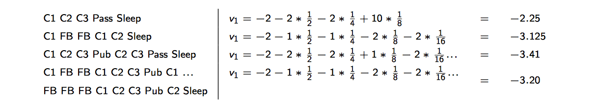
The return is random, but the value function is not random, rather, it is expectation of all samples' return.
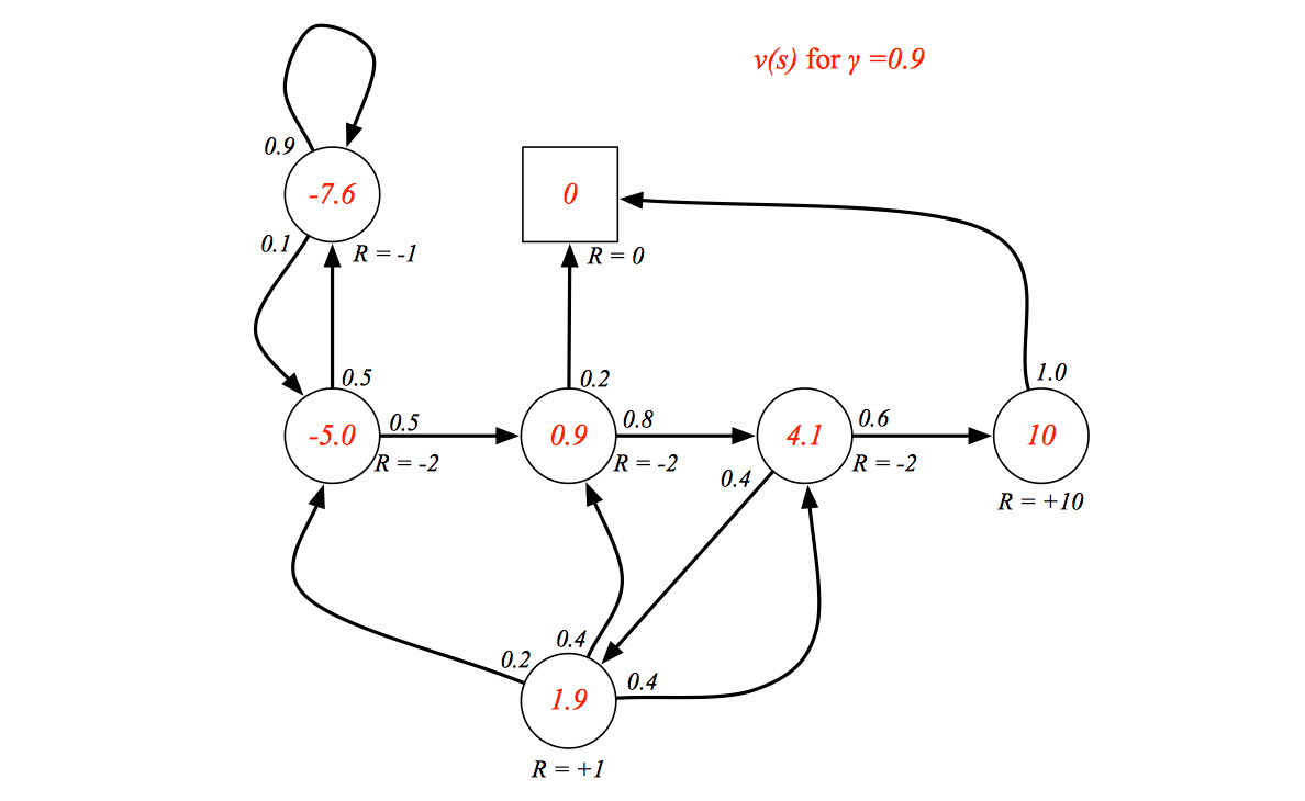
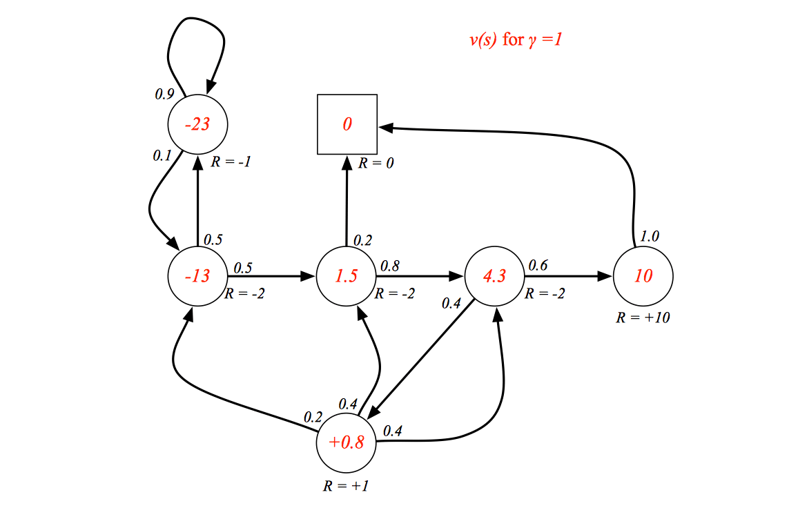
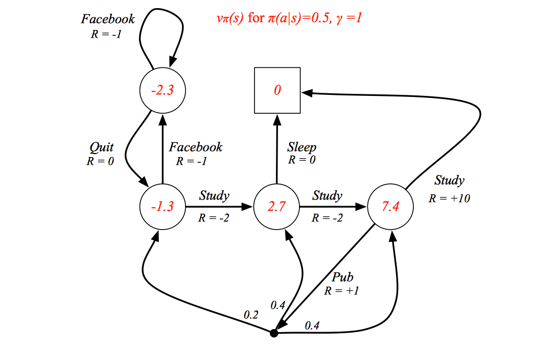
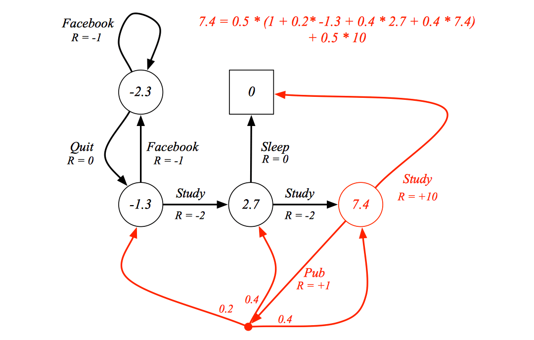
Let's see the example of state value function:
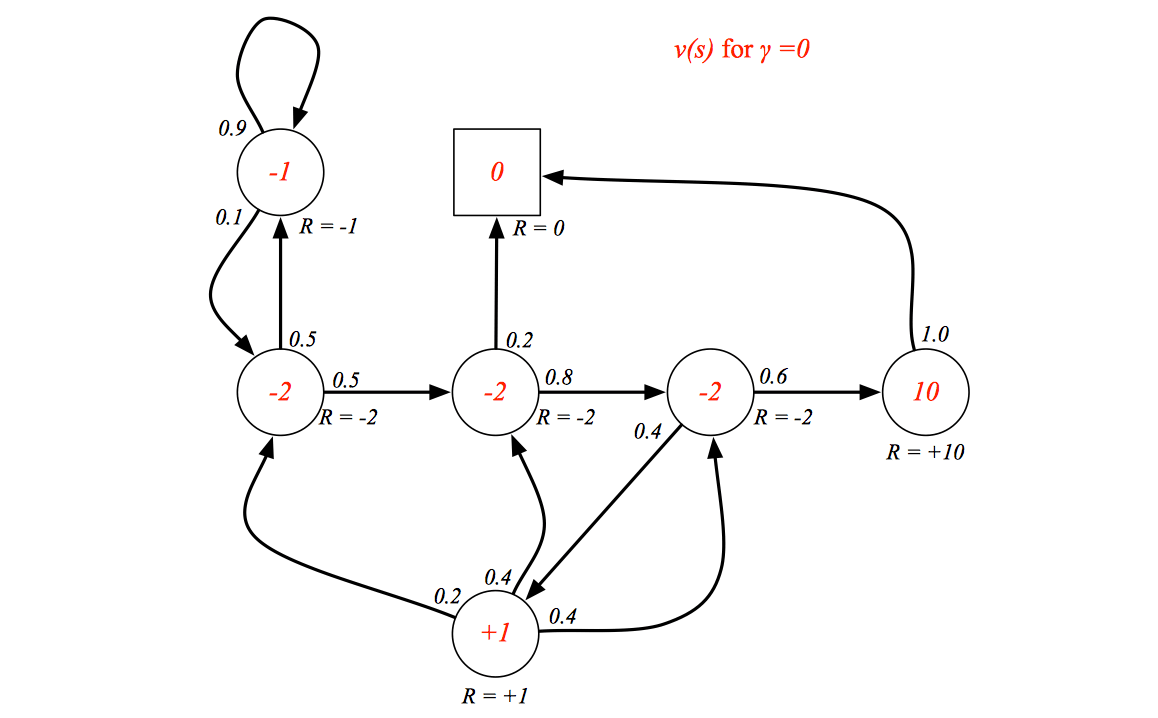
When \(\gamma = 0\), the value function just consider the reward of current state no matter how it changes future.
Bellman Equation for MRPs
The value function can be decomposed into two parts:
- immediate reward \(R_{t+1}\)
- discounted value of successor state \(\gamma v(S_{t+1})\)
So as to we can apply dynamic programming to solve the value function.
Here is the demonstration: \[ \begin{align} v(s) & = \mathbb{E}[G_t|S_t=s] \\ & = \mathbb{E}[R_{t+1}+\gamma R_{t+2}+\gamma^2 R_{t+3}+...|S_t=s] \\ &= \mathbb{E}[R_{t+1}+\gamma(R_{t+2}+\gamma R_{t+3}+...)|S_t=s]\\ &= \mathbb{E}[R_{t+1}+\gamma G_{t+1}|S_t=s]\\ &= \mathbb{E}[R_{t+1}+\gamma v(S_{t+1})|S_t=s] \end{align} \] Here we get: \[ v(s) =\mathbb{E}[R_{t+1}+\gamma v(S_{t+1})|S_t=s]=R_{t+1}+\gamma\mathbb{E}[ v(S_{t+1})|S_t=s] \] We look ahead one-step, and averaging all value function of next possible state:
 \[
v(s) = R_s+\gamma\sum_{s'\in S}P_{ss'}v(s')
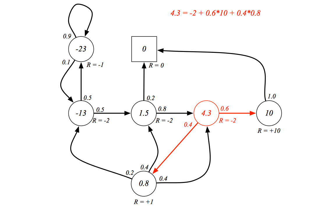
\] We can use the Bellman equation to vertify a MRP:
\[
v(s) = R_s+\gamma\sum_{s'\in S}P_{ss'}v(s')
\] We can use the Bellman equation to vertify a MRP:
Bellman Equation in Matrix Form
The Bellman equation can be expressed concisely using matrices, \[ v = R + \gamma Pv \] where \(v\) is a column vector with one entry per state: \[ \begin{bmatrix} v(1) \\ \vdots \\ v(n) \end{bmatrix}=\begin{bmatrix} R_1 \\ \vdots \\ R_n \end{bmatrix}+\gamma \begin{bmatrix} P_{11} & \cdots & P_{1n} \\ \vdots & \ddots & \vdots \\ P_{n1} & \cdots & P_{nn} \end{bmatrix}\begin{bmatrix} v(1) \\ \vdots \\ v(n) \end{bmatrix} \] Because the Bellman equation is a linear equation, it can be solved directly: \[ \begin{align} v & = R+\gamma Pv \\ (I-\gamma P)v& =R \\ v &= (I-\gamma P)^{-1}R \end{align} \] However, the Computational complexity is \(O(n^3)\) for \(n\) states, because of the inverse operation. This method can be applied to solve small MRPs.
There are many iterative methods for large MRPs, e.g.
- Dynamic programming
- Monte-Carlo evaluation
- Temporal-Difference learning
So far with MRP, all we want to do is to make decisions, so let's move on Markov Decision Process, which we actually using in RL.
Markov Decision Process
A Markov decision process (MDP) is a Markov reward process with decisions. It is an environment in which all states are Markov.
Definition
A Markov Decision Process is a tuple \(<S, A,P,R,\gamma>\)
- \(S\) is a finite set of states
- \(A\) is a finite set of actions
- \(P\) is a state transition probability matrix, \(P^a_{ss'}=\mathbb{P}[S_{t+1}=s'|S_t=s, A_t=a]\)
- \(R\) is a reward function, \(R^a_s=\mathbb{E}[R_{t+1}|S_t=s,A_t=t]\)
- \(\gamma\) is a discount factor \(\gamma \in[0,1]\)
Example
Red marks represents the actions or decisions, what we want to do is to find the best path that maximize the value function.
Policy
Formally, the decision can be defined as policy:
Definition
A policy π is a distribution over actions given states, \[ \pi(a|s)=\mathbb{P}[A_t=a|S_t=s] \]
A policy fully defines the behaviour of an agent.
Note that MDP policies depend on the current state (not the history), i.e. policies are stationary (time-independent), \(A_t~\pi(\cdot|S_t), \forall t>0\).
An MDP can transform into a Markov process or an MRP:
Given an MDP \(\mathcal{M}=<\mathcal{S,A,P,R}, \gamma>\) and a policy \(\pi\)
The state sequence \(<S_1 , S_2 , ... >\) is a Markov process \(<\mathcal{S, P}^π>\)
The state and reward sequence \(<S_1 , R_2 , S_2 , …>\) is a Markov reward process \(<\mathcal{S,P}^\pi,\mathcal{R}^\pi,\gamma>\) where, \[ \mathcal{P}^\pi_{s,s'}=\sum_{a\in\mathcal{A}}\pi(a|s)P^a_{ss'} \]
\[ \mathcal{R}^\pi_s=\sum_{a\in\mathcal{A}}\pi(a|s)\mathcal{R}^a_s \]
Value Function
There are two value functions: the first one is called state-value function which represents the expected return following policy \(\pi\), the other is called action-value function which measures the goodness/badness of an action following policy \(\pi\).
Definition
The state-value function \(v_π (s)\) of an MDP is the expected return starting from state \(s\), and then following policy π \[ v_\pi(s)=\mathbb{E}_\pi[G_t|S_t=s] \]
Definition
The action-value function \(q_π (s, a)\) is the expected return starting from state \(s\), taking action \(a\), and then following policy \(π\) \[ q_\pi(s,a)=\mathbb{E}_\pi[G_t|S_t=s,A_t=a] \]
Example
Bellman Expectation Equation
The state-value function can again be decomposed into immediate reward plus discounted value of successor state, \[ v_\pi(s)=\mathbb{E}_\pi[R_{t+1}+\gamma v_\pi(S_{t+1})|S_t=s] \] The action-value function can similarly be decomposed, \[ q_\pi(s,a)=\mathbb{E}_\pi[R_{t+1}+\gamma q_\pi (S_{t+1},A_{t+1})|S_t=s,A_t=a] \] Bellman Expectation Equation for \(V_π\)
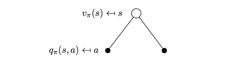 \[
v_\pi(s)=\sum_{a\in\mathcal{A}}\pi(a|s)q_\pi(s,a)
\] The look-ahead approach is taking an action and computing its reward, all we need to do is to averaging all possible actions' rewards, which is equal to current state-value.
\[
v_\pi(s)=\sum_{a\in\mathcal{A}}\pi(a|s)q_\pi(s,a)
\] The look-ahead approach is taking an action and computing its reward, all we need to do is to averaging all possible actions' rewards, which is equal to current state-value.
Bellman Expectation Equation for \(Q_π\)
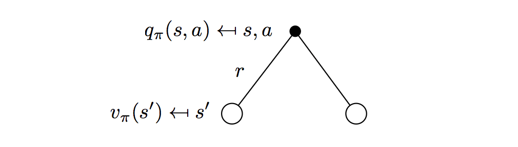 \[
q_\pi(s,a)=\mathcal{R}_s^a + \gamma \sum_{s'\in\mathcal{S}}P^a_{ss'}v_\pi(s')
\] It is identical to the immediate reward of taking action \(a\) plus the average of the reward/value of all possible states which the action could lead to.
\[
q_\pi(s,a)=\mathcal{R}_s^a + \gamma \sum_{s'\in\mathcal{S}}P^a_{ss'}v_\pi(s')
\] It is identical to the immediate reward of taking action \(a\) plus the average of the reward/value of all possible states which the action could lead to.
Bellman Expectation Equation for \(V_π\)
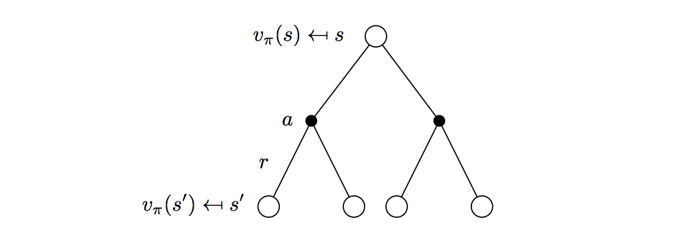 \[
v_\pi(s)=\sum_{a\in\mathcal{A}}\pi(a|s)(\mathcal{R}^a_s+\gamma\sum_{s'\in\mathcal{S}}P^a_{ss'}v_\pi(s'))
\] This is a two-step look-ahead approach, just combining the last two equations.
\[
v_\pi(s)=\sum_{a\in\mathcal{A}}\pi(a|s)(\mathcal{R}^a_s+\gamma\sum_{s'\in\mathcal{S}}P^a_{ss'}v_\pi(s'))
\] This is a two-step look-ahead approach, just combining the last two equations.
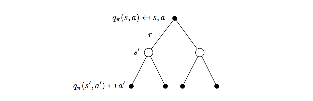 \[
q_\pi(s,a)=\mathcal{R}^a_s+\gamma\sum_{s'\in\mathcal{S}}P^a_{ss'}\sum_{a'\in\mathcal{A}}\pi(a'|s')q_\pi(s',a')
\] Example: State-value function
\[
q_\pi(s,a)=\mathcal{R}^a_s+\gamma\sum_{s'\in\mathcal{S}}P^a_{ss'}\sum_{a'\in\mathcal{A}}\pi(a'|s')q_\pi(s',a')
\] Example: State-value function
Bellman Expectation Equation (Matrix Form)
The Bellman expectation equation can be expressed concisely using the induced MRP, \[ v_\pi=R^\pi+\gamma P^\pi v_\pi \] with direct solution \[ v_\pi=(I-\gamma P^{\pi-1})^{-1}R^\pi \] Optimal Value Function
Definition
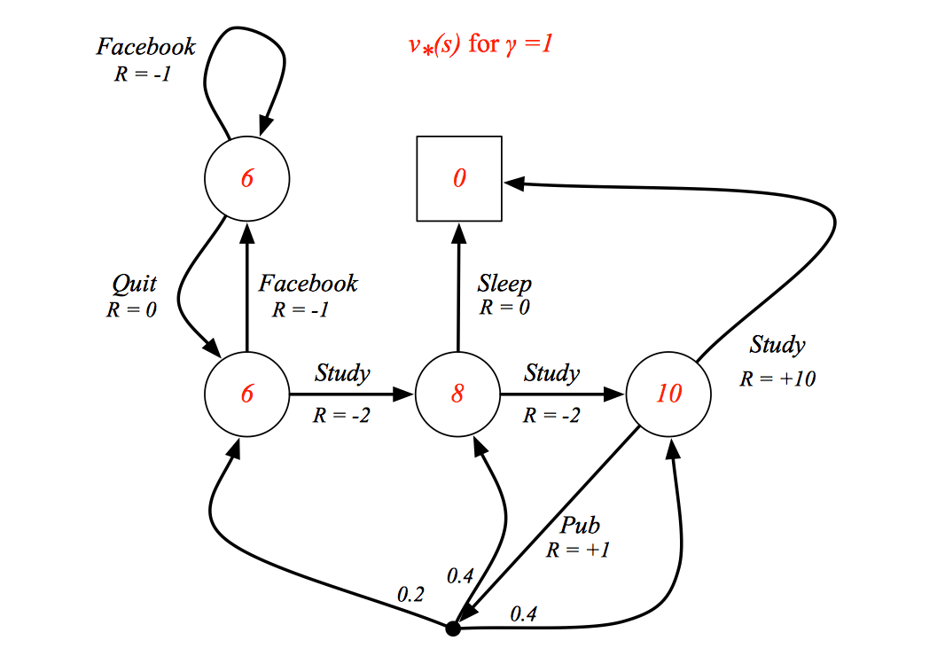
The optimal state-value function \(v_∗(s)\) is the maximum value function over all policies \[ v_\ast(s)=\max_{\pi}v_\pi(s) \] The optimal action-value function \(q_∗ (s, a)\) is the maximum action-value function over all policies \[ q_\ast(s,a)=\max_\pi q_\pi(s,a) \]
The optimal value function specifies the best possible performance in the MDP.
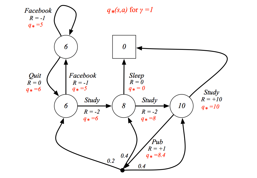
If we know the \(q_*(s,a)\), we "solve" MDP because we know what actions should take at each state to maximize the reward.
Example
Optimal Policy
Define a partial ordering over policies \[ \pi≥\pi'\ if\ v_\pi(s)≥v_{\pi'}, \forall s \]
Theorem
- There exists an optimal policy \(π_∗\) that is better than or equal to all other policies,, \(\pi_* ≥ \pi, \forall \pi\)
- All optimal policies achieve the optimal value function, \(v_{pi_*}=v_*(s)\)
- All optimal policies achieve the optimal action-value function, \(q_{\pi_*}(s,a)=q_*(s,a)\)
Finding an Optimal Policy
An optimal policy can be found by maximising over \(q_∗ (s, a)\),
\[ \pi_\ast(a|s)=\begin{cases} 1\ if\ a=\arg\max_{a\in\mathcal{A}}q_\ast(s,a) \\ 0 \ otherwise \end{cases} \]
There is always a deterministic optimal policy for any MDP. So if we know \(q_∗ (s, a)\), we immediately have the optimal policy.
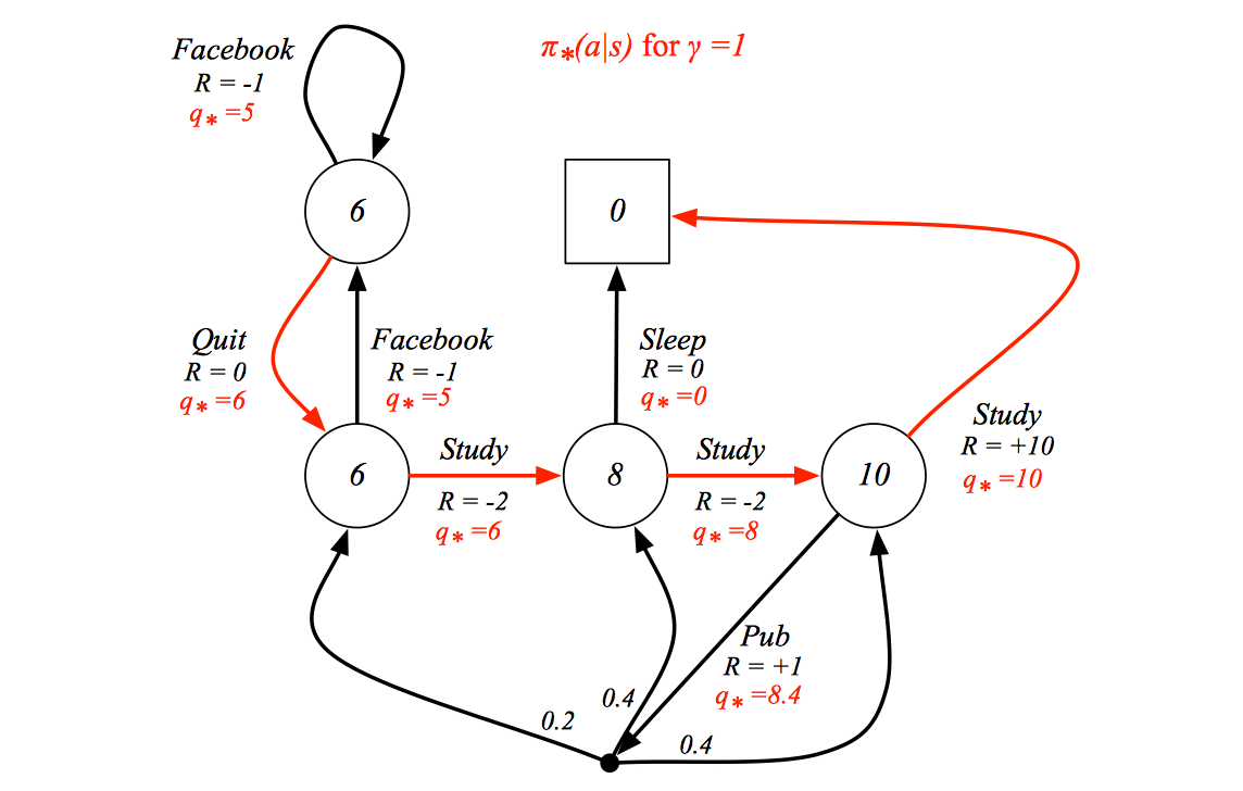
The optimal policy is highlight in red.
Bellman Optimality Equation
The optimal value functions are recursively related by the Bellman optimality equations:
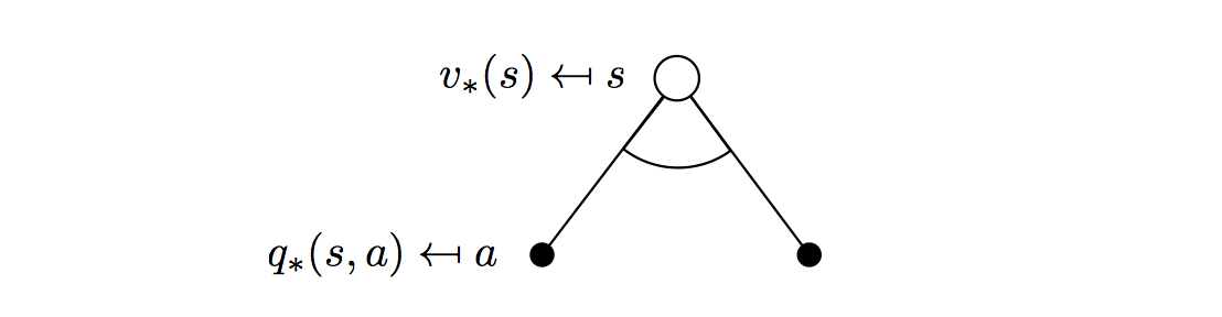
\[v_\ast(s)=\max_aq_\ast(s,a)\]

\[q_\ast(s,a)=\mathcal{R}^a_s+\gamma\sum_{s'\in\mathcal{S}}\mathcal{P}^a_{ss'}v_\ast(s')\]
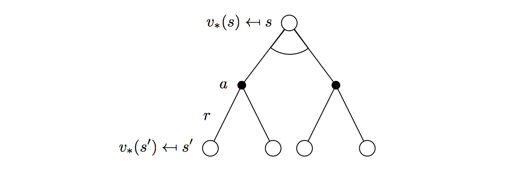
\[v_\ast(s)=\max_a\mathcal{R}^a_s+\gamma\sum_{s'\in\mathcal{S}}\mathcal{P}^a_{ss'}v_\ast(s')\]
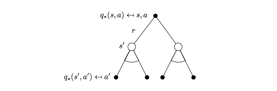
\[q_\ast(s,a)=\mathcal{R}^a_s+\gamma\sum_{s'\in\mathcal{S}}P^a_{ss'}\max_{a'}q_\ast(s',s)\]
Example

Solving the Bellman Optimality Equation
Bellman Optimality Equation is non-linear, so it is not able to be sovle as solving linear equation. And there is no closed from solution (in general).
Many iterative solution methods
- Value Iteration
- Policy Iteration
- Q-learning
- Sarsa
End. Next note will introduce how to solve the Bellman Optimality Equation by dynamic programming.